
In our previous blog post we discussed the purpose of a thread pool, various approaches to implementing a thread pool, along with a simulation model describing thread pool implementations in MariaDB and Percona Server. In this post we will look into another methodology of tuning the thread pool size, namely the adaptive Hill Climbing algorithm.
Similarity and difference between the two approaches can be commonly characterized as follows. In the previous post, the output of the given $\mathrm{TPSize}$ was calculated by a model invocation, where model is a standalone program. In this blog post, the output of the given $\mathrm{TPSize}$ is taken from a running database server in real-time and is immediately used for further tuning of the thread pool. So the main difference can be described as offline and online optimization, respectively.
Preface
The problem of the optimal thread pool size choice has continued to be an actual and important over the past few decades. The main goal of such optimization is maximizing throughput on the one hand, and minimizing resource consumption on the other hand. Adaptive solutions to this problem have been under active development during the last years. This blog post gives an overview of a successful application of those solutions to MySQL thread pool, which, however, does not limit its commonality for other software systems. The thread pool implementations in MariaDB and Percona Server were taken as a basis. The well-known Hill Climbing algorithm was used, while background and signal processing procedures produce data for taking decisions. This post contains several algorithmic heuristics and refinements to get realistic results for different types of workloads, differentiating it on criteria of whether the workload is heavy/low and CPU-bound/IO-bound. It is shown that performance improvement reaches more than 40% due to the optimal choice of the thread pool size with the adaptive approach. Finally, we provide proposals on further application of methods based on AI and machine learning for multi-dimensional optimizations.
The optimal value of $\mathrm{TPSize}$ depends on multiple factors in a complex way:
- Number of client requests
- Number of CPU cores
- Amount of memory
- Response time (request duration)
So how do you choose an optimal $\mathrm{TPSize}$? Guide [15] suggests the following:
The size computation takes into account the number of client requests to be processed concurrently, the resource (number of CPUs and amount of memory) available on the machine and the response times required for processing the client requests. Setting the size to a very small value can affect the ability of the server to process requests concurrently, thus affecting the response times since requests will sit longer in the task queue. On the other hand, having a large number of worker threads to service requests can also be detrimental because they consume system resources, which increases concurrency. This can mean that threads take longer to acquire shared structures, thus affecting response times.
There are simple expressions, repeated in many works (for example [11] and [16]), which give an intuitively clear way to choose a rather good approximation in many cases. The first one is:
\[N_{threads} = N_{cores}\cdot(1 + \frac{W}{S})\]where
- $N_{threads}$ – number of threads;
- $N_{cores}$ – number of available cores;
- $W$ – waiting time, that is the time spent waiting for IO bound tasks to complete;
- $S$ – service time, that is the time spent being busy;
- $\frac{W}{S}$ – ratio, that is often called the blocking coefficient.
The second one uses a fundamental result from the queuing theory. Little’s law says that the number of requests in a system equals the rate at which they arrive multiplied by the average amount of time it takes to service an individual request: $N=λ * W$. We can use Little’s law to determine the thread pool size. All we have to do is to measure the rate at which requests arrive and the average amount of time to service them. We can then plug those measurements into Little’s law to calculate the average number of requests in the system.
These assumptions were good enough for small software systems, but they are insufficient on the level of large industrial applications. Indeed, although they require to collect dynamic run-time information, they cannot be used to maximize throughput, because they know nothing about it. Nothing in them guarantees that we get an extremum point of the “concurrency level – throughput” dependency, and possible performance loss can be notable. But what do we know about that dependency? Why can we say that the task of looking for an optimum point is sensible? Why can too few threads be a bad choice, or vice versa, why can too many threads be a bad choice as well? How that dependency behaves itself in general? The following table illustrates the answer.
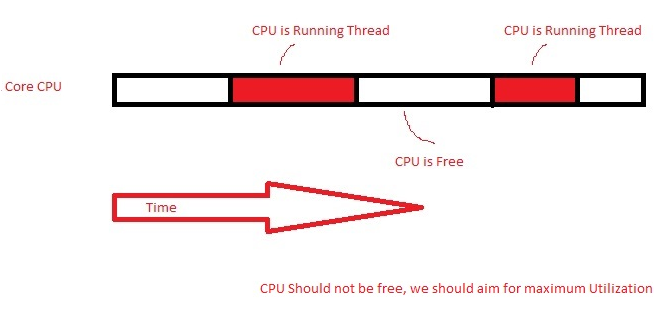 Too few threads: Reduce the ability of the server to process requests concurrently, thus affecting the response times since requests will sit longer in the task queue. CPU is free, but there are no threads to utilize it. Too few threads: Reduce the ability of the server to process requests concurrently, thus affecting the response times since requests will sit longer in the task queue. CPU is free, but there are no threads to utilize it. |
 Too many threads: Firstly, the overhead of context switching. Secondly, threads compete for system resources, thus taking longer to acquire shared structures and affecting response times. Too many threads: Firstly, the overhead of context switching. Secondly, threads compete for system resources, thus taking longer to acquire shared structures and affecting response times. |
We can see the two typical patterns of the learning dependency on figures 1 and 2.
| Figure 1: inherent to high connections (heavy load) | Figure 2: inherent to low connections (light load) |
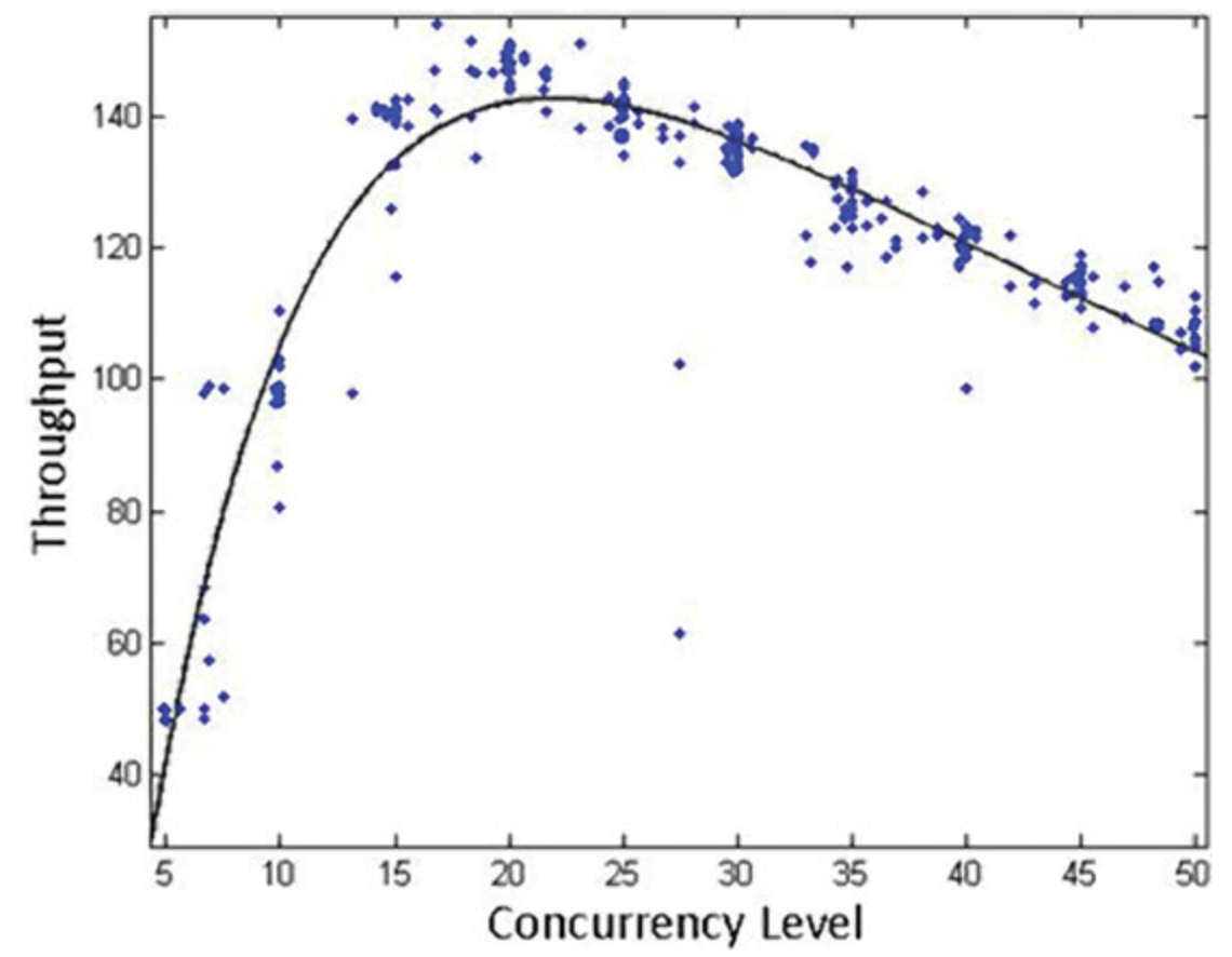 First grows (threads are utilizing CPUs), then falls (threads interfere with each other). First grows (threads are utilizing CPUs), then falls (threads interfere with each other). |
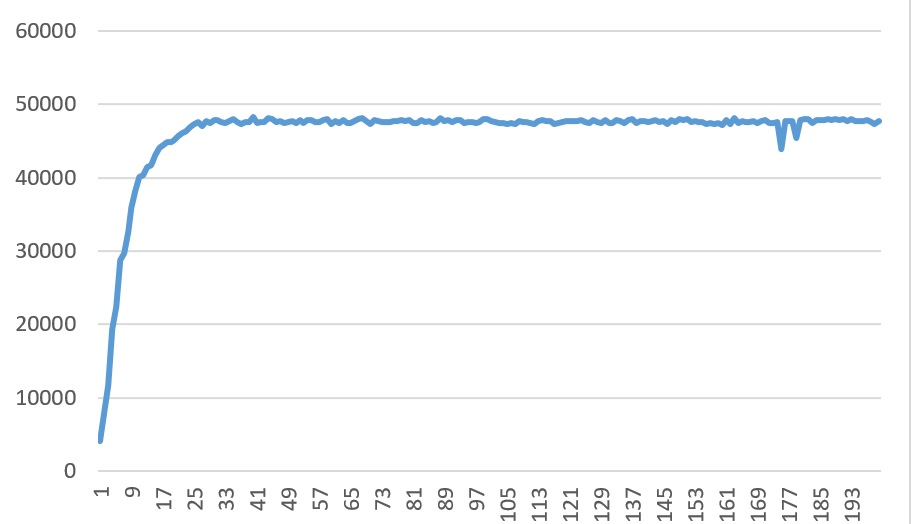 First grows (threads are utilizing as many CPUs as the light load allows), then constant from the “knee” point (no work items for other threads, they are idle and useless). First grows (threads are utilizing as many CPUs as the light load allows), then constant from the “knee” point (no work items for other threads, they are idle and useless). |
A good example when manually adjusting the thread pool size may improve performance in some workloads, while decreasing it in other workloads can be found here [3]. That’s why it is important for the thread pool to be able to adapt itself to changes in concurrency and workloads.
Adaptive Approach
So how to explore that knowledge? More precisely, what would be an effective approach to dynamically adapt $\mathrm{TPSize}$ in order to increase throughput while minimizing the amount of used threads? An adaptive approach will help us solve this problem and it is based on the Hill Climbing [9] optimization method. If you have never heard of it before, below is a brief explanation.
Hill Climbing In General: What Is It?
The Hill Climbing method is an optimization technique that is able to build a search trajectory in the search space until reaching the local optimum. It can be considered as a general class of heuristic optimization algorithms that deal with the following optimization problem. There is a finite set $X$ of possible configurations. Each configuration is assigned a non-negative real number called cost or, in other words, a cost function is defined as: $f : X \rightarrow R$. For each configuration $x \in X$, a set of neighbors $\eta(x) \subset X$ is defined. Let’s assume without restriction of generality that our goal is to maximize the cost function. The aim of the search is to find $x_{max} \in X$ maximizing the cost function $f(x), f(x_{max})=max{f(x) : x \in X}$ by moving from one neighbor to another depending on the cost difference between the neighboring configurations.
Let us list the typical steps of Hill Climbing in more details. Let’s assume for generality that the configuration is not a scalar but a vector, so we optimize the vector value.
- Step 1. Initialization of algorithm. Randomly create one candidate solution $\overrightarrow{x_{0}}$, depending on the length $\overrightarrow{x}$.
- Step 2. Evaluation. Create a cost function $f(\overrightarrow{x_{0}})$ to evaluate the current solution. The first iteration is as follows:
- Step 3. Mutation. Mutate the current solution $\overrightarrow{x_{*}}$ by one and evaluate the new solution $\overrightarrow{x_{i}}$.
- Step 4. Selection. If the value of the cost function for the new solution is better than for the current solution, replace as follows:
- Step 5. Termination. When there is no improvement in cost function after a few iterations.
The key step which determines the variety of the Hill Climbing heuristics is step 3 which is essentially mutate the current solution. How to mutate? It depends on what a researcher has thought up, proven and proposed. And as we will see further in this post when examining our problem, step 4 is also not quite deterministic.
Note a very important limitation of Hill Climbing: it converges to the nearest (as a rule) local optimum by its nature; it cannot be applied to a global optimum search. That is why the most appropriate application area for it are convex and concave cost functions.
State-of-the-art of the Hill Climbing family of algorithms in the middle of 90s of the last century can be found in the fundamental work [12]. Theoretical development of basic algorithms has been continued in the current century. A special stochastic version of Hill Climbing was proposed in [2] to overcome the problem of getting stuck to a local optimum. [10] extends the application area of Hill Climbing to such kind of problems as the hierarchical composition problem in order to choose the most appropriate neighbors for build blocks. A noticeable innovation was proposed in [23]. The main idea is that not only the search direction of the mutation is chosen randomly, but the subject area itself where we look for something is probabilistic. Thus, we improve the current solution not with probability one! Perhaps, this approach could be used after proper thinking for our problem too.
The variety of applied problems where Hill Climbing has been applied is very wide. Let’s note some interesting papers. [17] is devoted to the Graph Drawing problem. It addresses the problem of finding a representation of a graph that satisfies a given aesthetic objective, for example, embedding of its nodes in a target grid. Educational paper [20] considers Hill Climbing with respect to such well-known tasks of discrete optimization as scheduling with constraints (do not interfere on class-room access, on time of pupils’ groups, on time of lecturers); the problem of eight queens; traveling salesperson problem and others. It has been shown that Hill Climbing provides some advantages compared to the more classical methods, for example, limited amount of memory (because only the current state is stored) and ease of implementation. [4] applies Hill Climbing to cryptoanalysis, in particular, to the problem of recovering the internal state of the Trivium cipher. [8] considers permutation-based combinatorial optimization problems, such as the Linear Ordering problem and the Quadratic Assignment problem. [1] studies the problem of cluster analysis of Internet pages: how to map two or more pages on the same cluster. Authors solved two dualistic tasks: finding the minimum distance between each document in the dataset with cluster centroids and maximizing the similarity between each document with cluster centroids. Finally, [14] gives an example of Hill Climbing for continuous multi-dimensional problem of PID (Proportional-Integral-Derivative) tuning, where the aim is to tune the controller when control loop’s process value walks on significant excursion from the set point. The features of this task are more than one dependent variable and a very large search space.
Going back to thread pools, what is a configuration and what is a cost function for them? The configuration consists of one value which is $\mathrm{TPSize}$. The cost function returns the average throughput over a given time period with a given $\mathrm{TPSize}$, expressed for the database server in transactions per second (TPS). We can already describe our general plan in the following way: we observe and measure over time the changes in throughput as a result of adding or removing threads, then decide whether to add or remove more threads based on the observed throughput degradation or improvement. But how to do that?
First of all, let’s note two fundamental aspect of our subject area:
- the cost function is not exactly defined. As a database server is a very complex system influenced by many varying factors, two values measured over two different time periods will never match. We can only say whether the difference is statistically valuable or not. This is a bad aspect;
- the cost function is concave (see figures 1 and 2 again). That is why Hill Climbing can be applied in principle, and it only remains to decide how to apply it. This is a good aspect.
To make the decision, we have to remember about our goals:
-
- Primary goals:
-
- maximize throughput measured in completed transactions per second;
-
- minimize thread pool size for pattern 2;
-
- ensure convergence for both patterns from any initial value of the thread pool size;
-
- Secondary goals:
-
- detect a significant change in the workload and reset the iteration process;
-
- minimize the convergence time;
-
- minimize the overhead of a dynamic thread pool resizing;
-
- make implementation configurable by the user with meaningful parameters.
It should be noted that the most significant results in the adaptive thread pool approach over the last decade were obtained by Microsoft researchers. We will refer mostly to that work below.
Hill Climbing and Thread Pool: Control Theory
In this subsection we consider the technique described in papers [6] and [7]. It resembles gradient descent method [18], although strictly speaking it is not. The fact is that one iteration of the gradient descent changes all components of the configuration vector, however Hill Climbing changes only one of them in accordance with the chosen direction. But since configuration for the thread pool problem is one value, we can consder in fact the control theory technique as a gradient descent method after all. The iterative procedure (mutation) is the following:
\[x_{k+1} = x_{k} + sign(\Delta_{km})\lceil a_{km}|\Delta_{km}| \rceil \\ \Delta_{km} = \frac{\overline{y}_{km}-\overline{y}_{k-1}}{x_{km}-x_{k-1}} \\ a_{km} = e^{-s_{km}}\frac{g}{\sqrt{k+1}}\]where
- $\overline{y_{k-1}}$ is the value of throughput (cost function), calculated at $x_{k-1}$;
- $ \overline{y_{km}}$ is the value of throughput (cost function), averaged over $m$ sequential calculations at $x_{k}$;
- $s_{km}$ is the standard deviation of the sample mean of throughput values collected at $x_{k}$;
- $g$ is the control gain, the default value is 5.
The term $\Delta_{km}$ can be thought of as a “gradient”. Results, usage experience and practical suggestions are described in [22].
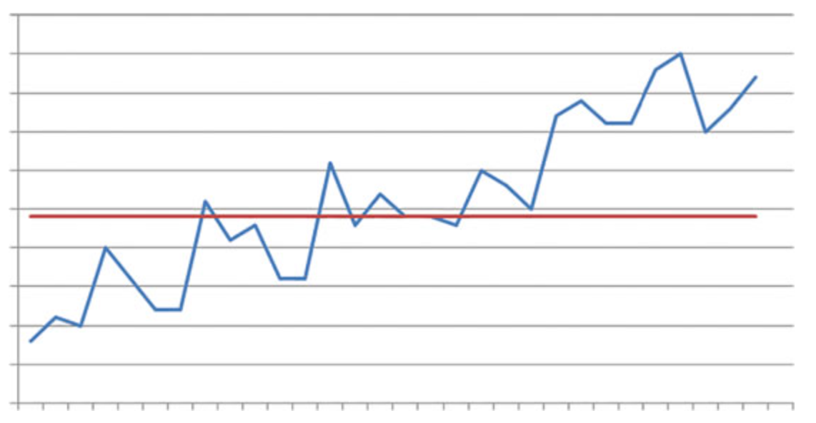
The main shortcoming of this method is that the measurements are noisy (Fig. 3), and the method does not handle it very well. The noise factor makes statistical information not representative of the actual situation, unless it’s taken over a large time interval, that is also unacceptable in practice.
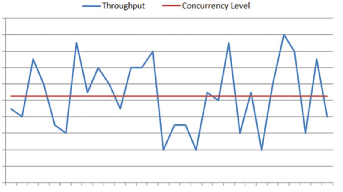 Figure 3: noise cost function: thread pool size is the constant, but throughput does fluctuate
[5] says the following about this method:
Its use was particularly problematic because of the difficulty in detecting small variations or extracting changes from a very noisy environment over a short time. The first problem observed with this approach is that the modeled function isn’t a static target in real-world situations, so measuring small changes is hard. The next issue, perhaps more concerning, is that noise (variations in measurements caused by the system environment, such as certain OS activity, garbage collection and more) makes it difficult to tell if there’s a relationship between the input and the output, that is, to tell if the throughput isn’t just a function of the number of threads. In fact, in the thread pool, the throughput constitutes only a small part of what the real observed output is—most of it is noise.
That is why in this method iterations turn into random walks often and do not bring performance any closer to the optimum point.
In this regard, it is worth mentioning the paper [21], where a simplified version of the described approach is proposed. The diagram of state transitions (Fig. 4) gives an idea of it.
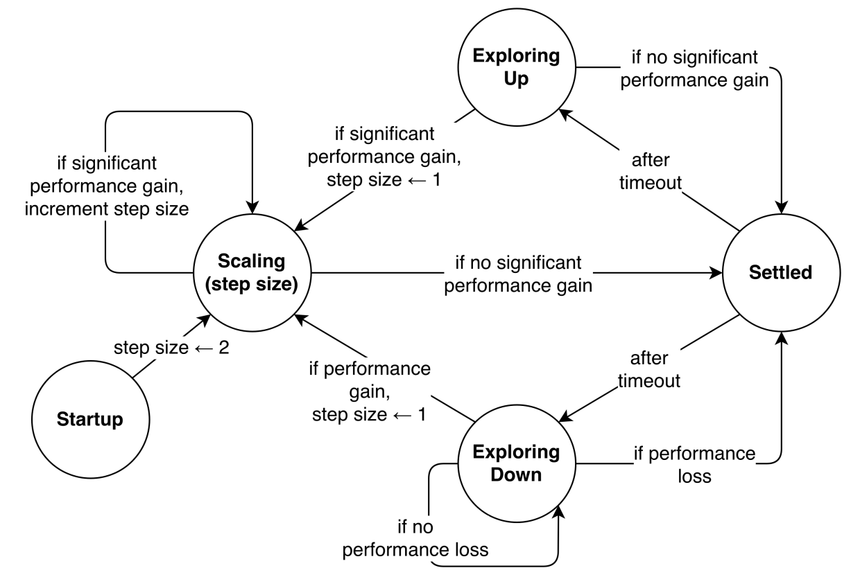 Figure 4: A simplified version of the control theory approach
In theory, this approach is reasonable, but in practice it suffers even more than the previous one from the same shortcomings due to the mutation and selection algorithms being too primitive. Let’s move on to the next methodology.
Hill Climbing and Thread Pool: Signal Processing
This approach is briefly described in [5] without details. The key idea is that we treat the input (concurrency level) and output (throughput) as signals. If we input a purposely modified concurrency level as a “wave” with known period and amplitude, and then look for that original wave pattern in the output, we can separate noise from the actual effect of the input on throughput. We introduce a signal and then try to find it in the noisy output. This effect can be achieved by using techniques generally used for extracting waves from other waves or finding specific signals in the output. This also means that by introducing changes to the input, the algorithm is making decisions at every point based on the last small piece of input data. Algorithm uses a discrete Fourier transform, a methodology that gives information such as the magnitude and the phase of a wave. This information can then be used to see if and how the input affected the output.
Let’s describe the basic decisive idea of the signal processing technique. There are two data rows (waves), which are a sequence of $\mathrm{TPSize}$ values and the corresponding sequence of throughput values. So we have already performed the Mutation step of Hill Climbing by varying $\mathrm{TPSize}$. Now it is the time of the Selection step. We have to figure out the common trend: does throughput improve or degrade with increasing of $\mathrm{TPSize}$? In the former case we will move one step up to increase $\mathrm{TPSize}$, in the latter one we will one the step down to decrease it.
We calculate the first Fourier harmonic of the first raw and the first Fourier harmonic of the second raw, these are both some complex numbers:
\[c_{1} = \rho_{1} (\cos \varphi_{1} + i \sin \varphi_{1}) \\ c_{2} = \rho_{2} (\cos \varphi_{2} + i \sin \varphi_{2})\]Then calculate the real part of the ratio $\frac{c_{1}}{c_{2}}$:
\[Re(\frac{c_{1}}{c_{2}}) = \frac{\rho_{1}}{\rho_{2}} \cos(\varphi_{1} - \varphi_{2})\]We then look at the sign of the ratio. A positive ratio means that $\varphi_{1} - \varphi_{2} < \frac{\pi}{2}$, that is why both data rows oscillate in-phase and have the same trends. In that case we increase $\mathrm{TPSize}$. A negative ratio means that $\varphi_{1} - \varphi_{2} > \frac{\pi}{2}$, thus both data rows oscillate in antiphase. Therefore, an increase of the first corresponds to a decrease of the second. In this case we decrease $\mathrm{TPSize}$.
To sum up, the direction of $\mathrm{TPSize}$ adjustment is determined by the sign of the real part of the first harmonics’ ratio.
Our approach uses signal processing and it is loosely based on the open source code of .NET [25]. That original code is sketchy and useless in practice for real server systems.
Our solution
The “true” behavior of the cost function in production database servers is hidden from a superficial view. Not to mention that the function itself changes in one way or another due to changes in the workload and the OS environment. That is why in order to get useful and applicable solution in practice we must identify and resolve many important issues, mainly to reject those artifacts which are caused not by $\mathrm{TPSize}$ adjustment. Let’s start from our states and transitions (Fig. 5).
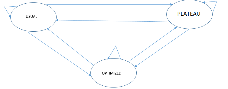 Figure 5: states and transitions
- Usual – iterations belonging to either increasing or decreasing parts of the curve to get closer to the optimal point;
- Plateau – iterations belonging to the constant part of the curve to get closer to the “knee” point;
- Optimized – no iterations, because we are on the optimal point. Сheck if the input has changed and reinit the search, if so.
We can see that transitions are possible between arbitrarily ordered state pairs, so, the graph is fuly connected. It is also important to note that algorithms and conditions of transitions are the engine of our solution as well as signal processing formulas.
The architecture of our adaptive thread pool module as a function call graph is shown on Fig. 6.
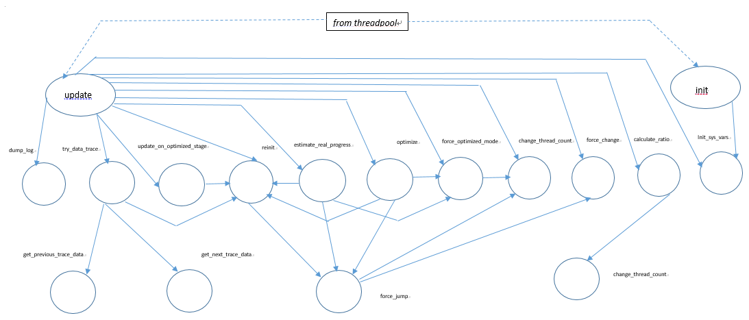 Figure 6: the adaptive thread pool module: the function call graph
Explanations of some important functions are:
init()– initialization of the Hill Climbing class properties, memory allocation of inner data structures;update()– implements the main iterative procedure and calls all auxiliary algorithms;dump_log()– prints debug information to a file in a structured way, can be disabled by a system variable;reinit()– restart the search of the optimal thread pool size when some external conditions are changed.reinit()cases are:- when the caller is
update_on_optimized_stage(): an exit from theOPTIMIZEDmode; - when the caller is
estimate_real_progress(): a false transition to theOPTIMIZEDmode; - when the caller is
optimize(): a false transition to theOPTIMIZEDmode; - when the caller is
try_data_trace(): a workload change is detected, the curve has changed; - when the caller is
update():- the thread pool size has been changed manually by a user;
- no connections;
- an unnaturally steep decline of throughput.
- when the caller is
Our own algorithm customizations
In this subsection we list some heuristics and mini-solutions that help to reach the declared goals on the one hand, and to compensate some computational artifacts of Hill Climbing with respect to the thread pool on the other hand.
False transition to the OPTIMIZED mode
The condition is: \(\mathrm{TPSize_{new}} – N_{connections} > 20\) (a configurable parameter). It makes no sense to have more threads than the number of concurrent connections. A small excess is allowed, but it should not be higher than a certain value.
False jump
The condition is: $\frac{N_{connections}}{\mathrm{TPSize_{new}}} < 0.2$ (a configurable parameter). The same logic as in the previous item is used. If the adjusted $\mathrm{TPSize}$ value exceeds the number of connections by a certain margin, we reject it.
Flexible step adjustment in the PLATEAU mode
This feature is applied when we move from the right to the left in the PLATEAU mode to find the “knee” point. The original rule $\mathrm{TPSize_{new}} = \frac{\mathrm{TPSize_{old}}}{2}$ is too coarse and results in large deviations to the left from the knee point. We have to provide a smaller value of jump down for lower \mathrm{TPSize}.
Let’s consider $2N$ reference points. Then we can propose the following formula:
\[\mathrm{TPSize_{new}} = \mathrm{TPSize_{old}}\cdot(0.5 + \sum_{i=1}^{N} k_{2i-1}\cdot e^{-k_{2i}\cdot\mathrm{TPSize_{old}}})\]For $N=1$, we chose two points \((10; 8)\) and \((20; 15)\) and calculated from the equation system $k_{1}=0.36$ and $k_{2}=0.018$. So the smaller is the value of $\mathrm{TPSize_{old}}$, the larger is the distance between $\mathrm{TPSize_{new}}$ and $\frac{\mathrm{TPSize_{old}}}{2}$.
Workload change detection
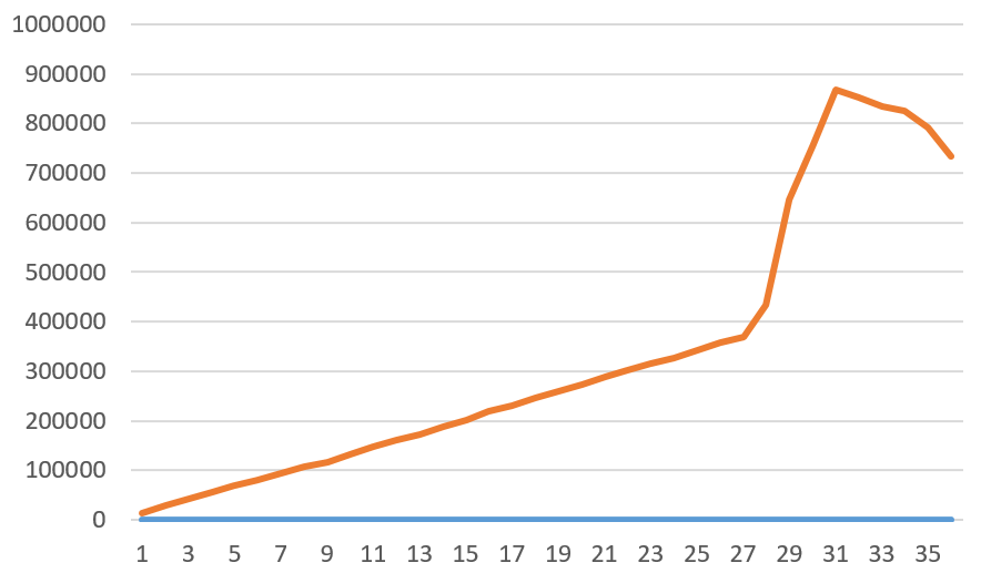
As we mentioned above, one of the reasons of the model re-initialization is “a workload change is detected, the curve has changed”. But how do we detect that? In other words, how does our approach perform with heterogeneous workloads and changing requests submission rate? Sometimes it’s hard to tell whether an improvement was a result of a change in concurrency or due to another factor such as workload fluctuations. That is why an improvement observed in a time interval may not even be related to the change in concurrency level (figure 7 helps to illustrate this issue).

The idea is simple. When the algorithm does its job, we store the calculated pairs $(\mathrm{TPSize}; \mathrm{throughput})$. When the first element of the next pair occurs between the two already known neighbor points, we predict the second element in accordance with some interpolation method, for example, even by a linear interpolation. The heuristic we apply here is that if actual throughput is too far from the predicted one, and such situation has repeated twice, then the cost function has changed and we have to re-initialize the algorithm. Fig. 8 illustrates this feature.
Entering and exiting the OPTIMIZED mode
Steps to enter and exit the OPTIMIZED mode are the following:
- Fix the throughput, the number of connections and request the average request latency when we enter the
OPTIMIZEDmode. - Check these data on each time interval (in the
update()function call) - If one of them deviated more than a certain threshold, defined by a configuration parameter, the
OPTIMIZEDmode is no longer applicable.
Overhead of the dynamic thread pool resizing
Using features of the MySQL thread pool implementations this is not a problem. This thread pool consists of some number of thread groups that is just $\mathrm{TPSize}$. Among with other fields, each thread group structure contains the following fields:
pollfd, which is a file descriptor for listening events with theio_poll_wait()API and extraction of input requests;mutexto protect group fields from concurrent access.
Thus, when we increase $\mathrm{TPSize}$, creating missing file descriptors (if any) is all we need to do; if we decrease $\mathrm{TPSize}$ we have nothing to do. Listing 1 illustrates that.
Listing 1.
void set_threadpool_size(uint size) {
  if (!threadpool_started) return;
  bool success = true;
  uint i = 0;
  for (i = 0; i < size; i++) {
    thread_group_t *group = &all_groups[i];
    mutex_lock(&group->mutex);
    if (group->pollfd == -1) {
      group->pollfd = io_poll_create();
      success = (group->pollfd >= 0);
      if (!success) {
        /*some message to log*/
        mutex_unlock(&all_groups[i].mutex);
        break;
      }
    }
    mutex_unlock(&all_groups[i].mutex);
  }
  if (success) group_count = size;
  else group_count = i;
}
Jumping down
The original signal processing variant of Hill Climbing for the adaptive thread pool can oscillate only forward from the current $\mathrm{TPSize}$ value, not backwards. That is why if the spectral analysis of two waves has shown an improvement, there no questions with the Selection step: we just add to the current $\mathrm{TPSize}$ value the current magnitude since that value has proven to be better. But what about degradation? It is clear that $\mathrm{TPSize}$ needs to be decreased, but how much? This question can be answered only with some plausible heuristics. The simplest and natural idea is to use the absolute value of the real part of the first harmonics ratio in a way to make the decrement value proportional. We can use the previously obtained correspondences between already made forward jumps and their real parts for scaling.
User configurable parameters for adaptive thread pool
For experimental purposes we introduce 33 new parameters to fine tune the Hill Climbing iteration process and decision making. Most of them will never need to be changed in production. The most important ones to tune or debug the module in rare cases:
hcm_hillclimbing_enabled– switch on/off the adaptive thread pool module. Default is false;hcm_log_enabled– switch on/off log file dumping. Default is false;wave_period– period of forced oscillation of the thread pool size. Default is 4;samples_to_wave_period_ratio– defines the history size of the previous thread pool size and throughput values, which are taken for consideration by the adaptive thread pool engine. Default is 8, so we take two vectors with 32 values each;hcm_period– the time interval in seconds between two sequential calls of theupdate()function. In other words, it is the sampling interval for the adaptive algorithm. Default value is 2;min_accepted_throughput– if the current throughput has dropped below this threshold, we suspend the adaptive thread pool module as using it is not practical. Default value is 300;hcm_eps– accuracy of the optimal value search. The optimal concurrency is considered as found, if the distance between the current upper and lower boundaries have become less thanhcm_eps. Default is 5;hcm_valuable_diff– the maximum deviation (in percent) of one value from another (either events per second or average latency). Default is 20%. Used to exit theOPTIMIZEDmode or to detect workload changes;hcm_ccs_valuable_progress– triggers a change in the thread pool size when the absolute accumulated sum of $Re(\frac{c_{1}}{c_{2}})$ reaches this threshold. Default is 0.2;hcm_max_thread_wave_magnitude– the upper boundary for $\mathrm{TPSize}$ oscillation magnitude, which we gradually increase fromhcm_min_thread_wave_magnitude(default is 10). If the specified magnitude has been reached, we conclude that there is no growing/falling trend and switch to thePLATEAUmode. Default is 80.
Testing
When it comes to testing of our Hill Climbing module it would be logical to check it first on some deterministic simple cost functions with an explicit and the only point of maximum like this (Fig. 9).
Such tests are needed to eliminate the most coarse bugs and estimate convergence time. We must convince that our Hill Climbing procedure converges to the optimum point from any initial value, either to the right or left from the optimum point. Until these tests are passed, there is no sense in testing on a real database server with a thread pool. The key features of such a simple test suite are the following:
- an artificially created table defining the cost function and matching one of two patterns. The correct answer is known in advance;
- a linear or spline interpolation in intermediate points;
- the hill climbing engine as a standalone program, not embedded into a database server;
- simple, fast and easy tests.
If all is OK with tests on simple framework it is time to move on to real database server with Sysbench framework. It was developed by Russian researcher Alexey Kopytov and described in many sources, for example, [13]. The goal of this testing is to try the adaptive thread pool on a real MySQL server with a synthetic workload that is close to realistic; to find possible artifacts; to refine auxiliary algorithmic features and finally, to evaluate performance improvements for different types of workloads. Base configuration is the following:
- HWSQL server 8.0;
- 10 tables with one million records in each;
- different workload profiles such as point select, read only and read write;
- different number of connections such as 1, 4, 16, 24, 32, 48, 64, 96, 128, 256, 512, 1024;
- 10-minute test duration for each concurrency level;
- the variable
hcm_log_enabledis switched on for subsequent exhaustive log file analysis.
The following hardware profile was used for Sysbench tests:
- Ubuntu 20.04, x86_64, GNU/Linux;
- Intel® Xeon® Gold 6151 CPU@3.00GHz;
- 72 CPUs;
- 628 Gb of memory.
It should be noted that the adaptive thread pool does not give a noticeable performance improvement for the sysbench/ps and sysbench/ro workloads as well as for CPU-bound workloads in general, although it minimizes $\mathrm{TPSize}$ for them, thus minimizing the resource usage for that kind of workloads. But for the sysbench/rw and sysbench/TPC-C workloads it improves performance by more than 40%. Let’s see in in our results.
Results
Before demonstrating the results of performance experiments let’s illustrate some profiling data, namely, the difference in distribution between Off-CPU time for CPU-bound and IO-bound workloads (Fig. 10, 11).
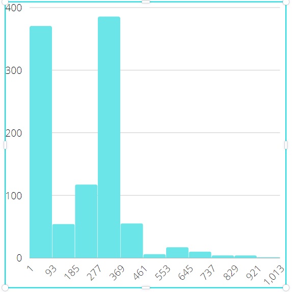 Figure 10: off-CPU time for CPU-bound workload Figure 10: off-CPU time for CPU-bound workload |
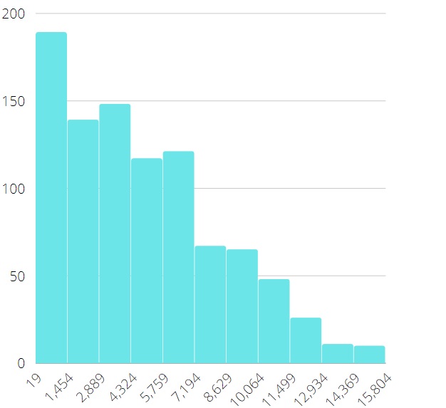 Figure 11: off-CPU time for IO-bound workload Figure 11: off-CPU time for IO-bound workload |
Off-CPU time is the time interval between the threadpool::wait_begin() and threadpool::wait_end() calls. As we can see comparing the data of the x-axis, that this time is 15 times higher for the IO-bound workload. And optimal $\mathrm{TPSize}$ much higher than the number of CPUs is typical for IO-bound workloads with longer off-CPU times. The optimal $\mathrm{TPSize}$ which is close to the number of CPUs is typical for CPU-bound workloads. This fact is confirmed by table below and explained in Fig. 12.
For each pair (connections; profile), three 10-minutes sysbench run were launched:
- With
hillclimbing_enabled=on, the thread pool size is 72 (the initial value). The result is the optimal value of $\mathrm{TPSize}$ (column opt); - With
hillclimbing_enabled=off, the thread pool size is 72 (a constant value). The result is the average throughput in queries per second (column usual); - With
hillclimbing_enabled=off, the thread pool size is opt (a constant value). The result is the average throughput in queries per second (column contr); - Column diff contains a diff of the contr column compared to the usual column.
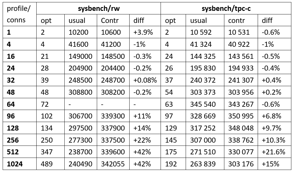 |
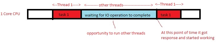 Figure 12: why extra threads are useful with IO-bound workload Figure 12: why extra threads are useful with IO-bound workload |
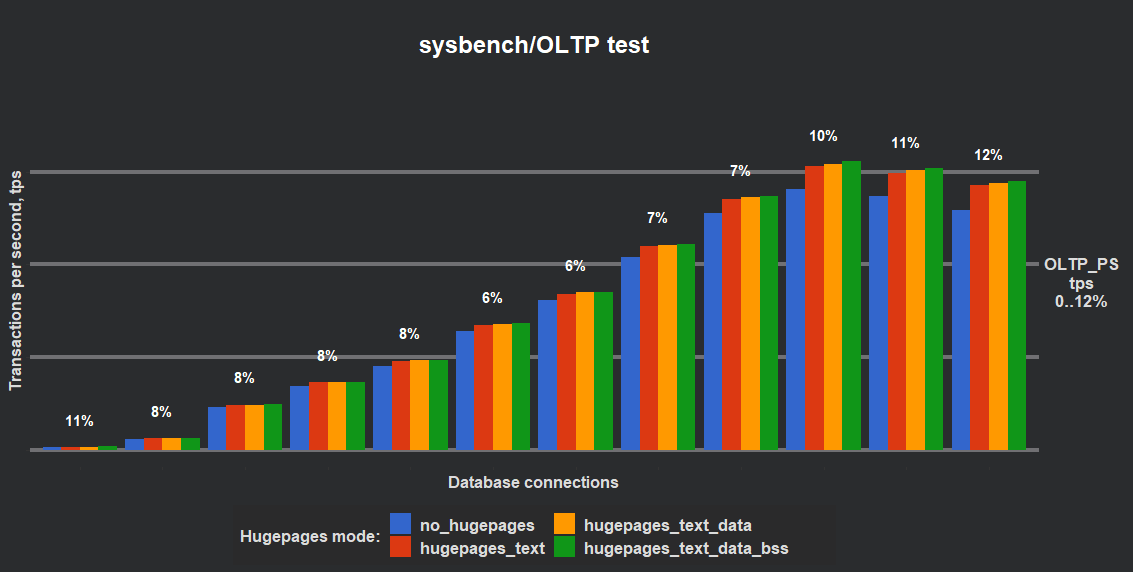
Figures 13 and 14 illustrate performance improvements provided by the adaptive thread pool for the sysbench/rw workload. The number of connections is depicted on the x-axis in both figures.
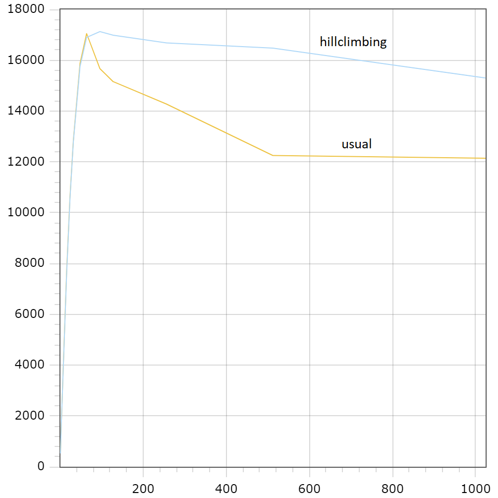 Figure 13: average throughput (transactions per second) Figure 13: average throughput (transactions per second) |
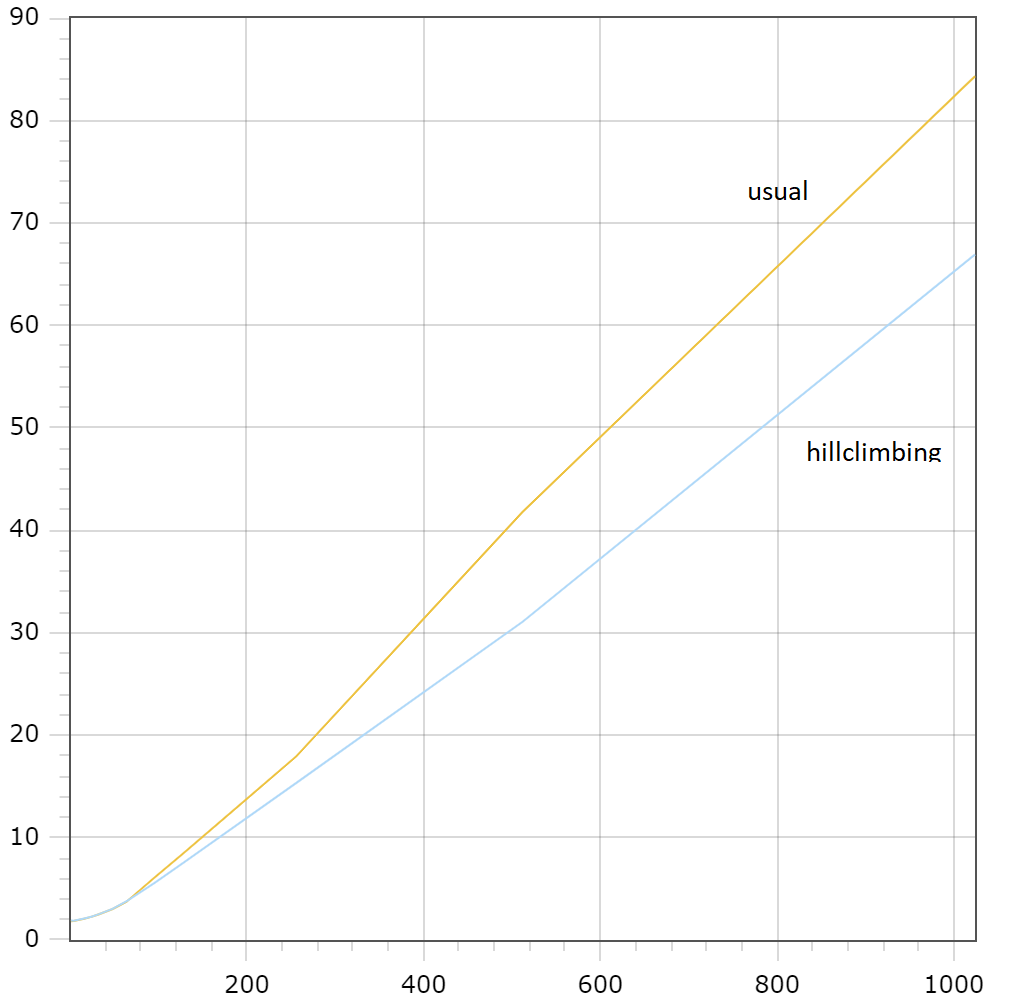 Figure 14: average latency (millisecond) Figure 14: average latency (millisecond) |
The fact that performance improvements on the pictures are slightly less than the ones declared in table should not be surprising because this experiment differs from the previous one. Pictures are built over 10-minute runs, where each one started from the same initial value and includes the time of hill climbing convergence. Thus, it worked with optimal $\mathrm{TPSize}$ not all of the time.
Figures 15 and 16 are equivalents of 13 and 14 for the sysbench/tpc-c workload.
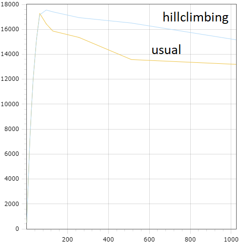 Figure 15: average throughput (transsactions per second) Figure 15: average throughput (transsactions per second) |
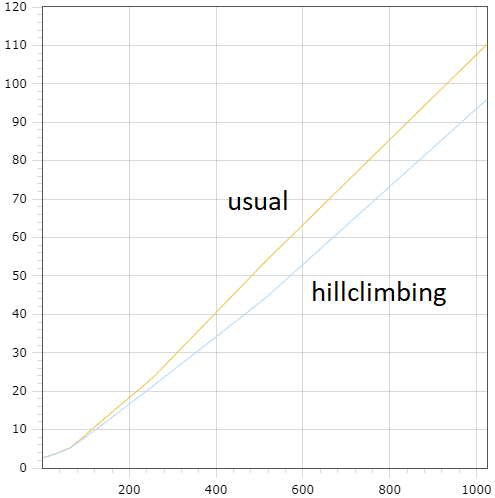 Figure 16: average latency (millisecond) Figure 16: average latency (millisecond) |
Figures 17 and 18 contain dependencies of the optimal $\mathrm{TPSize}$ value on various concurrency levels for different types of workload. These figures illustrate such feature of our solution as minimizing $\mathrm{TPSize}$ for low concurrency, which is more inherent to graphs on the right picture. We can see that even for the sysbench/ps and sysbench/ro workloads the algorithm finds the optimal $\mathrm{TPSize}$ value which is higher that the number of cores for high concurrency. Which is reasonable, because the found optimal values give a small, but still visible increase of performance for those workloads.
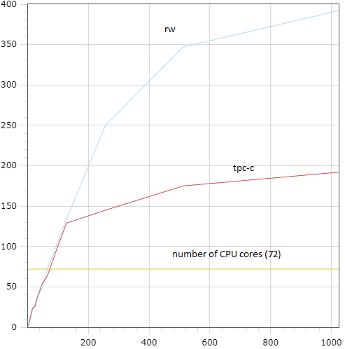 Figure 17: sysbench/rw and sysbench/tpc-c Figure 17: sysbench/rw and sysbench/tpc-c |
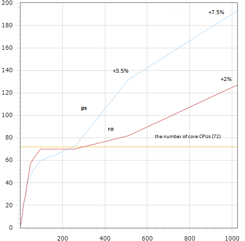 Figure 18: sysbench/ps and sysbench/ro Figure 18: sysbench/ps and sysbench/ro |
Generalization And Future Work
And finally a few words about machine learning (ML) approach in databases and how it relates to our solution. This approach has been actively researched in the last years [24]. The current state is the following. Some separate software module (for example, a thread pool) is configured by several parameters, chosen by developers or DBA. All combinations of those parameters as well as each of them in particular affects the output, which is some performance measure. Thus, if some tuple of parameter values gives the maximum performance, the goal is to find the optimal tuple of parameters. The optimal tuple varies in a wide range depending on various items, such as:
- server’s hardware configuration (number and types of CPU, volume of RAM and swap partition, etc.);
- operation system and job scheduling algorithms;
- current load from clients in the sense of quantity (concurrency levels);
- current load from clients in the sense of types (distribution of request lengths and availability of consumed resources, such as CPU and disk).
To find the optimal tuple on a given server multi-dimensional search set, the Hill Climbing method can be applied. Any found optimal tuple corresponds to some fixed workload on the given server. If we describe the profile of that workload more or less completely, we can expect that the next time when the profile will be approximately the same, we already know the optimal tuple. Just this idea is the cornerstone of the proposed approach.
The general plan is:
- profile the code in a proper way and collect workload data when the adaptive algorithm is active;
- put the found optimal tuple into the correspondence of collected data, thus getting a new record of the training dataset;
- when the training dataset will become large enough, we train our ML model on it, then try to apply this model before the adaptive algorithm completes its work.
So, collection of the workload profile test data for the ML model takes much less time than the convergence of the adaptive algorithm’s iterative process.
According to [19], we can perform ML procedures just in database by means of the proposed SQL extension. We do not need to address external ML tools after the extraction of training dataset from the database. It seems that when implemented, the results of that work will significantly improve the efficiency of the described approach.
Let’s give an example of a thread pool tuple:
- oversubscribe – defines the maximum number of active threads in one group;
- timer_interval – the time interval before activities of the
Timerthread; - queue_put_limit – wake or create a thread in queue_put(), if the number of active threads in the group is less or equal to this parameter;
- wake_top_limit – create a new thread in
wake_or_create_thread()only if the number of active threads in the group is less or equal to this parameter; - create_thread_on_wait – a boolean parameter define if a new thread should be created in
wait_begin(); - idle_timeout – the maximum time a thread can be in the idle state;
- listener_wake_limit – the listener thread wakes up an idle thread, if the number of active threads is less or equal to this parameter;
- listener_create_limit – the listener thread creates a new thread, if the number of active threads is less or equal to this parameter.
And a workload profile may look like this:
- the number of persistent connections;
- the number of CPUs (the return value of
getncpus()) - the latency of a new thread creation (timing of the
create_worker()function); - the number of active rounds in processing of a single request (from the start of the execution to the first
wait_begin()call + all rounds fromwait_end()towait_begin()+ the round from the lastwait_end()to the end of execution); - the duration of a single active round in a request execution;
- the duration of a single wait round in a request execution;
- the time interval between the end of a single request execution and the start of the next request execution in
io_poll_wait()for one connection.
References
1: L. M. Abualigah, E. S. Hanandeh, T. A. Khader, M. Otair, S. K. Shandilya, An Improved $\beta$-hill Climbing Optimization Technique for Solving the Text Documents Clustering Problem. – Current medical imaging reviews, vol. 14(4), 2020, pp.296-306.
2: M. A. Al-Betar, $\beta$-Hill climbing: an exploratory local search. – Neural Computing & Applications, vol.28, 2017, pp.153-168.
3: K. Bauskar, MariaDB thread pool and NUMA scalability (December 2021). – https://mysqlonarm.github.io/mdb-tpool-and-numa
4: J. Borghoff, L. R. Knudsen, K. Matusiewicz, Hill Climbing Algorithms and Trivium. – 17th International Workshop, Selected Areas in Cryptography (SAC) – 2010, Waterloo, Ontario, Canada, August 2010 (Springer, 2011), pp.57-73.
5: E. Fuentes, Concurrency – Throttling Concurrency in the CLR 4.0 Threadpool (September 2010). – https://docs.microsoft.com/en-us/archive/msdn-magazine/2010/September/concurrency-throttling-concurrency-in-the-clr-4-0-threadpool
6: J. L. Hellerstein, V. Morrison, E. Eilebrecht, Applying Control Theory in the Real World. – ACM’SIGMETRICS Performance Evaluation Rev., Volume 37, Issue 3, 2009, pp.38-42. doi: 10.1145/1710115.1710123.
7: J. L. Hellerstein, V. Morrison, E. Eilebrecht, Optimizing Concurrency Levels in the .NET Threadpool. – FeBID Workshop 2008, Annapolis, MD USA.
8: L. Hernando, A. Mendiburu, J. P. Lozano, Hill-Climbing Algorithm: Let’s Go for a Walk Before Finding the Optimum. – 2018 IEEE Congress on Evolutionary Computation (CEC), 2018, pp.1-7.
9: Hill climbing. – https://en.wikipedia.org/wiki/Hill_climbing
10: D. Iclanzan, D. Dumitrescu, Overcoming Hierarchical Difficulty by Hill-Climbing the Building Block Structure (February 2007). – https://arxiv.org/abs/cs/0702096
11: A. Ilinchik, How to set an ideal thread pool size (April 2019). – https://engineering.zalando.com/posts/2019/04/how-to-set-an-ideal-thread-pool-size.html
12: A. W. Johnson, Generalized Hill Climbing Algorithms for Discrete Optimization Problems. - PhD thesis, Virginia Polytechnic Institute and State University, Blacksburg, Virginia, October, 1996, 132 pp. - https://researchgate.net/publication/277791527_Generalized_Hill_Climbing_Algorithms_For_Discrete_Optimization_Problems
13: A. Mughees, How to benchmark performance of MySQL using Sysbench (June 2020). – https://ittutorial.org/how-to-benchmark-performance-of-mysql-using-sysbench
14: K. Nagarajan, A Predictive Hill Climbing Algorithm for Real Valued multi-Variable Optimization Problem Like PID Tuning. – International Journal of Machine Learning and Computing, vol.8, No.1, February, 2018. – https://ijmlc.org/vol8/656-A11.pdf
15: Oracle GlassFish Server 3.1 Performance Tuning Guide. – https://docs.oracle.com/cd/E18930_01/pdf/821-2431.pdf
16: K. Pepperdine, Tuning the Size of Your Thread Pool (May 2013). – https://infoq.com/articles/Java-Thread-Pool-Performance-Tuning
17: A. Rosete-Suarez, A. Ochoa-Rodriquez, M. Sebag, Automatic Graph Drawing and Stochastic Hill Climbing. – GECCO’99: Proceedings of the First Annual Conference on Genetic and Evolutionary Computing, vol. 2, July 1999, pp.1699-1706.
18: S. Ruder, An overview of gradient descent optimization algorithms (2016). – https://arxiv.org/abs/1609.04747
19: M. Schüle, F. Simonis, T. Heyenbrock, A. Kemper, S. Günnemann, T. Neumann, In-Database Machine Learning: Gradient Descent and Tensor Algebra for Main Memory Database Systems. – In: Grust, T., Naumann, F., Böhm, A., Lehner, W., Härder, T., Rahm, E., Heuer, A., Klettke, M. & Meyer, H. (Hrsg.), BTW 2019. Gesellschaft für Informatik, Bonn. pp. 247-266. – https://dl.gi.de/bitstream/handle/20.500.12116/21700/B6-1.pdf?sequence=1&isAllowed=y doi: 10.184.20/btw2019-16.
20: B. Selman, C. P. Gomes, Hill-climbing Search (2001). – https://www.cs.cornell.edu/selman/papers/pdf/02.encycl-hillclimbing.pdf
21: J. Timm, An OS-level adaptive thread pool scheme for I/O-heavy workloads. – Master thesis, Delft University of Technology, 2021. https://repository.tudelft.nl/islandora/object/uuid%3A5c9b4c42-8fdc-4170-b978-f80cd8f00753
22: M. Warren, The CLR Thread Pool ‘Thread Injection’ Algorithm (April 2017). – https://codeproject.com/Articles/1182012/The-CLR-Thread-Pool-Thread-Injection-Algorithm
23: J.-H. Wu, R. Kalyanam, P. Givan, Stochastic Enforced Hill-Climbing. – Proceedings of the 2013 IEEE International Conference on Systems, Man and Cybernetics, October 2013.
24: X. Zhou, J. Sun, Database Meets Artificial Intelligence. – IEEE Transactions on Knowledge and Data Engineering, May 2020. doi: 10.1109/TKDE.2020.2994641.
25: https://github.com/dotnet/coreclr/blob/master/src/vm/win32threadpool.cpp


Comments